Logistic regression analysis

Methods of Corpus Linguistics (class 6)

Mariana Montes

Outline

Introduction
Probabilities, odds and logit
Evaluation
Interactions
Random effects

Introduction

Set up code

set.seed(2022)
gonna <- tibble(variant = rep("gonna", 50), comp_length = rnorm(50, 6, 0.8),
                register = sample(c("formal", "informal"), 50, replace = TRUE, prob = c(0.1, 0.9)))
going_to <- tibble(variant = rep("going_to", 50), comp_length = rnorm(50, 3, 1.2),
                   register = sample(c("formal", "informal"), 50, replace = TRUE, prob = c(0.7, 0.3)))
gt <- bind_rows(gonna, going_to) %>%
  mutate(
    comp_length = if_else(comp_length > 1, comp_length, 1),
    variant = fct_relevel(variant, "gonna"),
    variant_num = as.numeric(variant)-1,
    register = fct_relevel(register, "informal"),
    source = factor(sample(letters, n(), replace = TRUE))
  )
m1 <- glm(variant ~ comp_length, data = gt, family = binomial(logit))
gt$fit1 <- m1$fitted.values
m2 <- glm(variant ~ comp_length + register, data = gt, family = binomial(logit))
gt$fit2 <- m2$fitted.values

gonna_plot <- ggplot(gt, aes(x = comp_length, y = variant_num)) +
  geom_point(size = 3) + ylim(0, 1) +
  labs(x = "Length of complement", y = "Choice of construction") +
  scale_y_continuous(breaks = c(0, 1), labels = c("gonna", "going to")) +
  theme_minimal(base_size = 20) + theme(aspect.ratio = 1)

gonna dataset

Code

kb_style(filter(gt, variant == "gonna"), "float_left")
kb_style(filter(gt, variant == "going_to"), "left")

variant	comp_length	register	source	fit1	fit2
gonna	6.72	formal	q	0.008	0.050
gonna	5.06	informal	x	0.348	0.137
gonna	5.28	informal	z	0.233	0.081
gonna	4.84	informal	i	0.480	0.221
gonna	5.74	informal	m	0.088	0.026
gonna	3.68	informal	f	0.946	0.861
gonna	5.15	informal	j	0.297	0.111
gonna	6.22	informal	p	0.027	0.007
gonna	6.60	informal	p	0.011	0.003
gonna	6.19	formal	c	0.029	0.174

variant	comp_length	register	variant_num	source	fit1	fit2
going_to	2.75	formal	1	g	0.995	0.999
going_to	4.22	formal	1	r	0.817	0.975
going_to	4.64	formal	1	x	0.608	0.929
going_to	4.77	formal	1	q	0.526	0.901
going_to	4.07	informal	1	f	0.869	0.691
going_to	1.78	formal	1	y	1.000	1.000
going_to	5.25	formal	1	p	0.251	0.723
going_to	4.29	informal	1	g	0.789	0.551
going_to	1.71	informal	1	h	1.000	0.999
going_to	1.00	formal	1	c	1.000	1.000

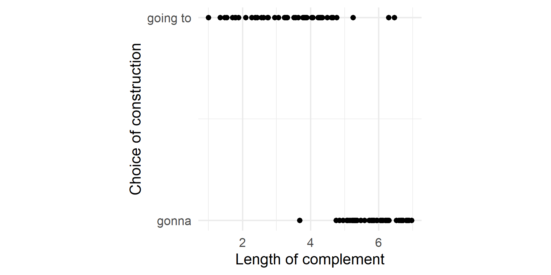
Scatterplot

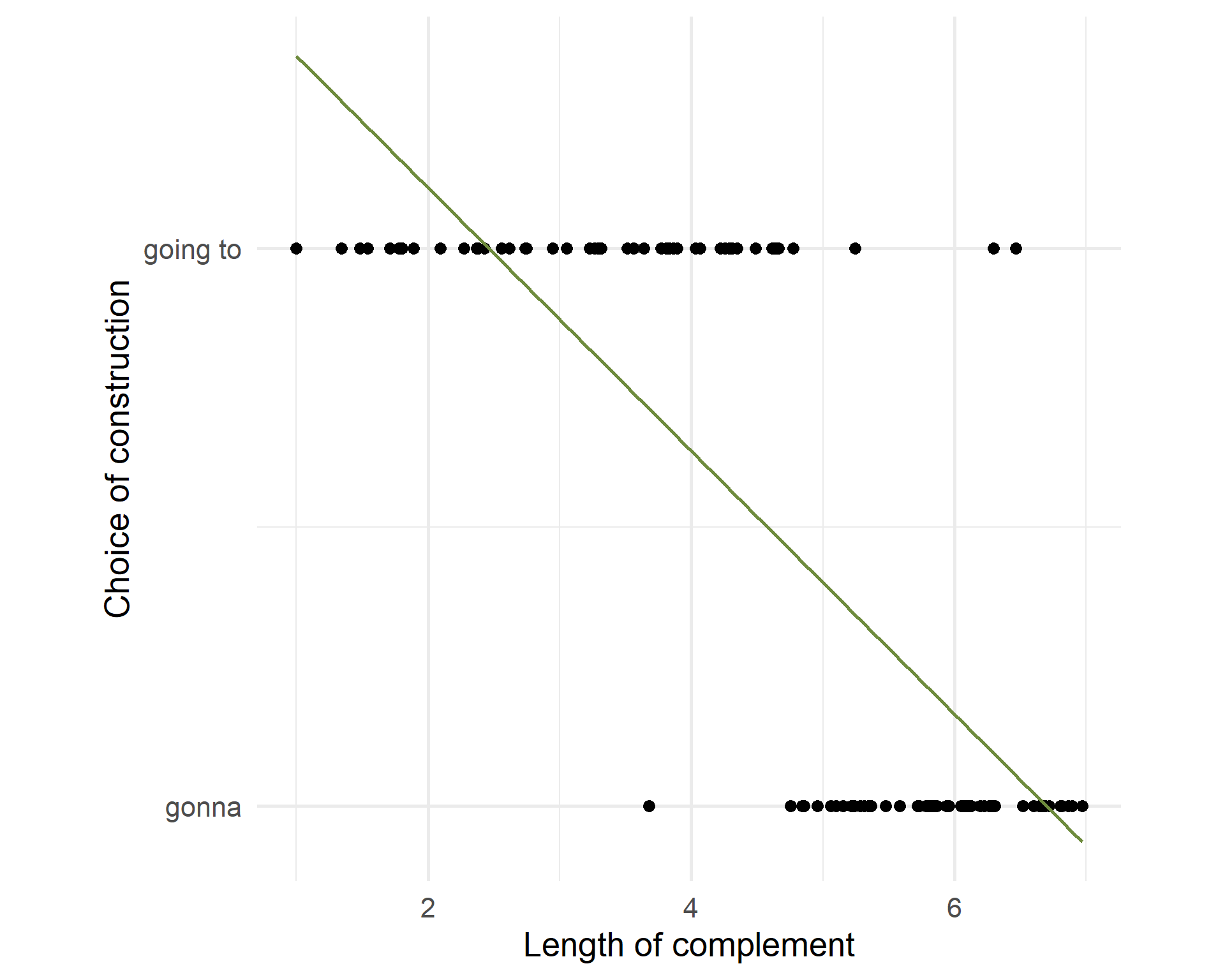
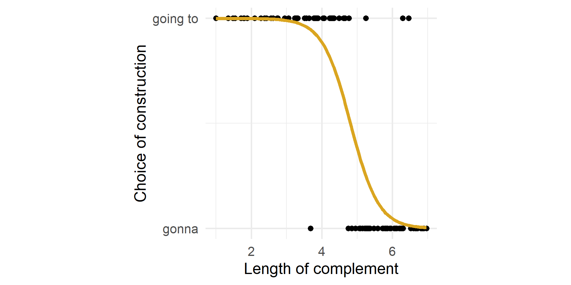
What is the relationship between the length of the complement and the choice of going to/gonna?

Code

gonna_plot

Linear fit

The relationship is not linear.

Code

gonna_plot + 
  geom_smooth(method = "lm", se = FALSE, color = "darkolivegreen4")

The residuals are not normally distributed.
Not all values are possible (probabilities go between 0 and 1).

Logistic fit

The fit has an S shape.

Code

gonna_plot +
  geom_line(aes(y = fit1), color = "goldenrod", size = 2)

Model

Code

summary(m2)


Call:
glm(formula = variant ~ comp_length + register, family = binomial(logit), 
    data = gt)

Deviance Residuals: 
    Min       1Q   Median       3Q      Max  
-1.9876  -0.2053  -0.0209   0.1067   2.1787  

Coefficients:
               Estimate Std. Error z value Pr(>|z|)    
(Intercept)      11.582      2.899    4.00  6.5e-05 ***
comp_length      -2.651      0.613   -4.32  1.5e-05 ***
registerformal    3.284      1.068    3.08   0.0021 ** 
---
Signif. codes:  0 '***' 0.001 '**' 0.01 '*' 0.05 '.' 0.1 ' ' 1

(Dispersion parameter for binomial family taken to be 1)

    Null deviance: 138.63  on 99  degrees of freedom
Residual deviance:  34.02  on 97  degrees of freedom
AIC: 40.02

Number of Fisher Scoring iterations: 7

Interpretation

Intercept

log odds of outcome (“going to”) when all predictors are at 0 (comp_length = 0).
odds = exp(11.582) = 107138
prob = odds/(odds+1) \(\approx\) 1

Coefficients

log odds ratios: positive increases chances of “going to”, negative of “gonna”.
odds ratio
- of comp_length = exp(-2.651) = 0.071
- of register = exp(3.284) = 26.676

The odds of going to vs gonna in the formal register are 26.676 times higher than those in the informal register, other variables being controlled for.

Probabilities, odds and logit

Probabilities

probs.

\(P\)
0 - 0.5 - 1
Number of successes divided by number of trials.

Odds

probs.

\(P\)
0 - 0.5 - 1
Number of successes divided by number of trials.

odds

\(\frac{P}{1-P}\)
0 - 1 - \(\infty\)
Probability of success divided by the probability of failure.
Undefined for \(P=1\).

Logit

probs.

\(P\)
0 - 0.5 - 1
Number of successes divided by number of trials.

odds

\(\frac{P}{1-P}\)
0 - 1 - \(\infty\)
Probability of success divided by the probability of failure.
Undefined for \(P=1\).

logit

\(\log\left(\frac{P}{1-P}\right)\)
\(-\infty\) - 0 - \(\infty\)
If positive, success is more likely; if negative failure is more likely.
Undefined for \(P=0\) and for \(P=1\).

Simulation

library(MASS) # to print fractions

probabilities <- c(1/c(7:2),
                   1-(1/c(3:7)))
probs <- tibble(
  P = probabilities,
  P_frac = as.character(fractions(P)),
  odds = P/(1-P),
  odds_frac = as.character(fractions(odds)),
  logit = log(odds)
)
kbl(probs) %>% kable_paper(font_size = 22) %>% 
  row_spec(6, bold = TRUE)

P	P_frac	odds	odds_frac	logit
0.143	1/7	0.167	1/6	-1.792
0.167	1/6	0.200	1/5	-1.609
0.200	1/5	0.250	1/4	-1.386
0.250	1/4	0.333	1/3	-1.099
0.333	1/3	0.500	1/2	-0.693
0.500	1/2	1.000	1	0.000
0.667	2/3	2.000	2	0.693
0.750	3/4	3.000	3	1.099
0.800	4/5	4.000	4	1.386
0.833	5/6	5.000	5	1.609
0.857	6/7	6.000	6	1.792

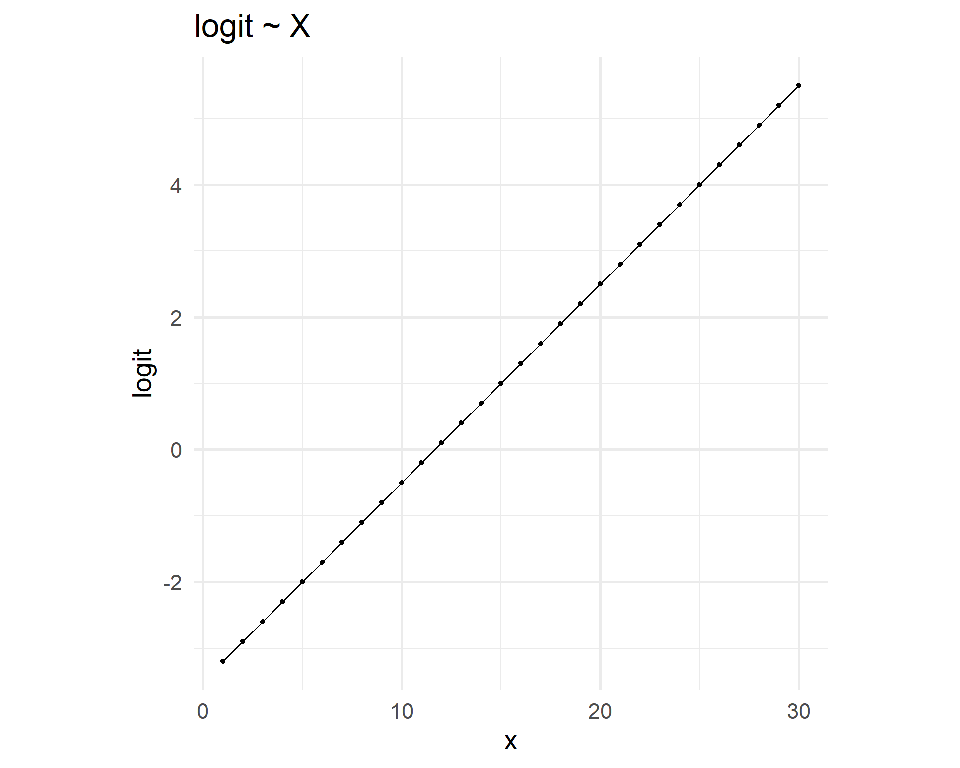
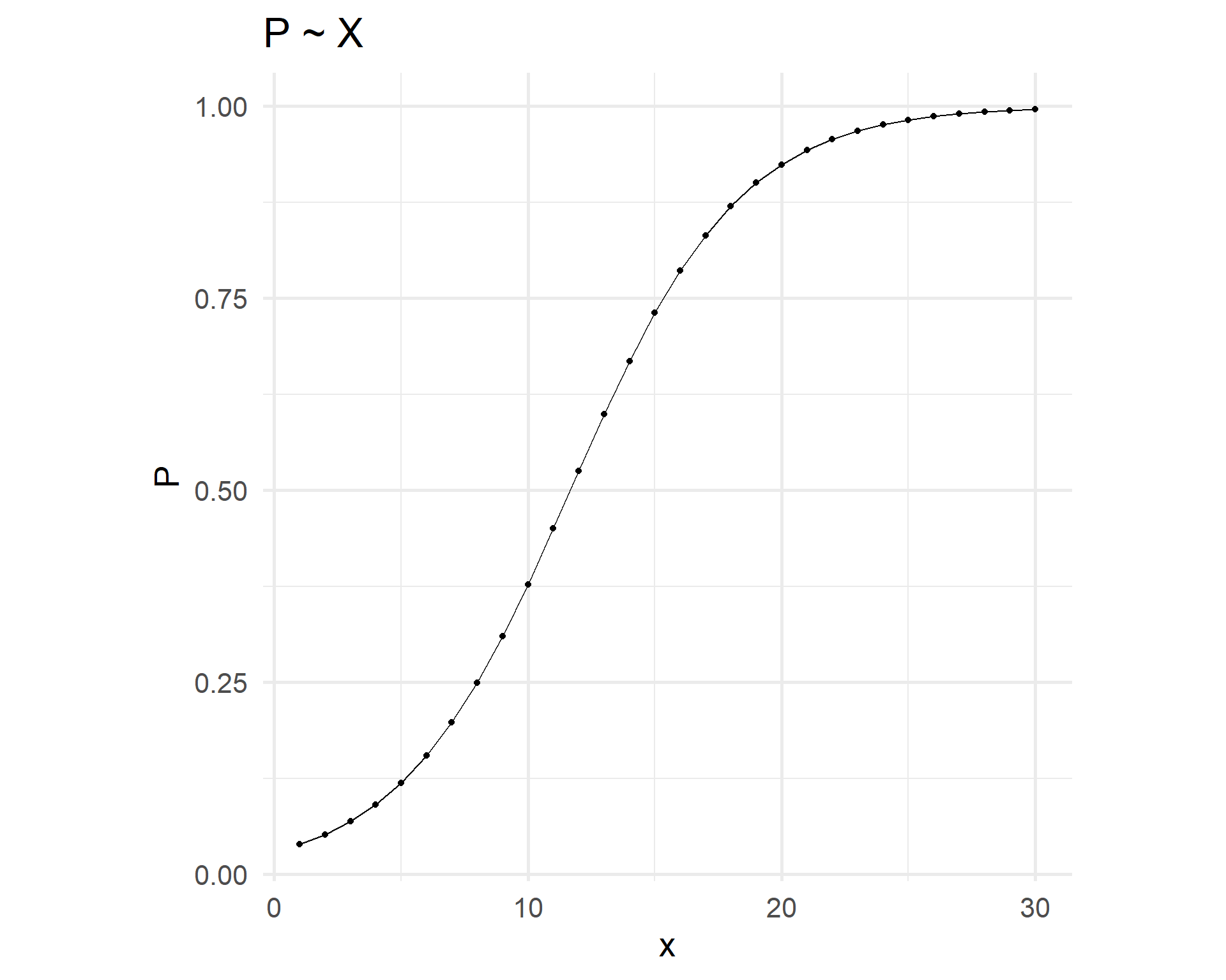
Linear vs logistic relationships

Linear relation logit ~ x entails logistic curve p ~ x.

Code

with_x <- tibble(x = 1:30, logit = -3.5 + 0.3*x, odds = exp(logit), P = odds/(1+odds))

Code

lnplot(with_x, x, logit, "logit ~ X")

Code

lnplot(with_x, x, P, "P ~ X")

Evaluation

Model

Code

summary(m2)


Call:
glm(formula = variant ~ comp_length + register, family = binomial(logit), 
    data = gt)

Deviance Residuals: 
    Min       1Q   Median       3Q      Max  
-1.9876  -0.2053  -0.0209   0.1067   2.1787  

Coefficients:
               Estimate Std. Error z value Pr(>|z|)    
(Intercept)      11.582      2.899    4.00  6.5e-05 ***
comp_length      -2.651      0.613   -4.32  1.5e-05 ***
registerformal    3.284      1.068    3.08   0.0021 ** 
---
Signif. codes:  0 '***' 0.001 '**' 0.01 '*' 0.05 '.' 0.1 ' ' 1

(Dispersion parameter for binomial family taken to be 1)

    Null deviance: 138.63  on 99  degrees of freedom
Residual deviance:  34.02  on 97  degrees of freedom
AIC: 40.02

Number of Fisher Scoring iterations: 7

Deviance

Null deviance: discrepancy between data and intercept-only model (like SST)
Residual deviance: discrepancy between data and fitted model (like SSE)

Computation

\(-2 \log(L)\) with \(L\) the likelihood of encountering the data if the model is true.

AIC (Akaike Information Criterion): corrected residual deviance (to compare models with different N. of predictors) - the smaller the better
Deviance residuals: contribution of each observation to the residual deviance.

Predicted probability

\[g(x) = \beta_0 + \beta_1x_1 + \beta_2x_2 + ...\]

Let’s predict the probability of going to when complement length is 4 and register is formal.

\[g(x) = 11.582 + -2.651\times 4 + 3.284 \times 1 = 4.26\]

odds = exp(4.26) = 70.802

\[P(x) = \frac{70.802}{70.802 + 1} = 0.986\]

Measures of predictive power

We take all pairs of observations in which the response variable is different (one of gonna, one of going to).

gt0 is what the model predicted for the “gonna” element.
gt1 is what the model predicted for the “going to” element.

Code

set.seed(0)
pred_power <- tibble(
  gt0 = sample(filter(gt, variant == "gonna")$fit2, 15, replace = FALSE),
  gt1 = sample(filter(gt, variant == "going_to")$fit2, 15, replace = FALSE))
kb_style(pred_power, n = 15)

gt0	gt1
0.011	0.999
0.221	1.000
0.009	0.999
0.050	1.000
0.021	0.895
0.001	1.000
0.793	1.000
0.006	0.942
0.090	0.998
0.265	1.000
0.006	0.514
0.019	1.000
0.174	0.093
0.111	0.420
0.003	1.000

C, D, T

C = concordant pair = prediction is higher for “going to” 😁
D = discordant pair = the prediction is higher for “gonna” ☹️
T = tie = the prediction is the same for both 😐

Code

pred_power <- pred_power %>%
  mutate(C = gt1 > gt0, D = gt0 > gt1, T = gt1 == gt0)
kb_style(pred_power, n = 15) %>%
  column_spec(3, background = spec_color(pred_power$C, option = "H", begin = 0.8, end = 0.45))

gt0	gt1	C	D	T
0.011	0.999	TRUE	FALSE	FALSE
0.221	1.000	TRUE	FALSE	FALSE
0.009	0.999	TRUE	FALSE	FALSE
0.050	1.000	TRUE	FALSE	FALSE
0.021	0.895	TRUE	FALSE	FALSE
0.001	1.000	TRUE	FALSE	FALSE
0.793	1.000	TRUE	FALSE	FALSE
0.006	0.942	TRUE	FALSE	FALSE
0.090	0.998	TRUE	FALSE	FALSE
0.265	1.000	TRUE	FALSE	FALSE
0.006	0.514	TRUE	FALSE	FALSE
0.019	1.000	TRUE	FALSE	FALSE
0.174	0.093	FALSE	TRUE	FALSE
0.111	0.420	TRUE	FALSE	FALSE
0.003	1.000	TRUE	FALSE	FALSE

C-value

Code

pred_power <- pred_power %>%
  summarize(C = sum(C), D = sum(D), T = sum(T))
kb_style(pred_power)

C	D	T
14	1	0

\[c = \frac{C+T/2}{C+D+T} = \frac{14+0/2}{14+1+0} = 0.933\]

Hmisc::somers2(gt$fit2, gt$variant_num)[["C"]]

[1] 0.984

Linear vs logistic regression

	Linear regression	Logistic regression
Response variable	Numerical	Categorical
Relationship between predictor estimate and response	Linear	Logistic¹
Fitting function	OSL (ordinary least squares)	MLE (maximum likelihood estimation)
Model comparison	F-test	AIC
Evaluation metric	\(R^2\)	\(C\)
Base R function	`lm()`	`glm()`

Interactions

What is an interaction?

When the effect of a predictor depends on the value of another predictor.

Formula: y ~ x1 + x2 + x1:x2 = y ~ x1*x2

Examples

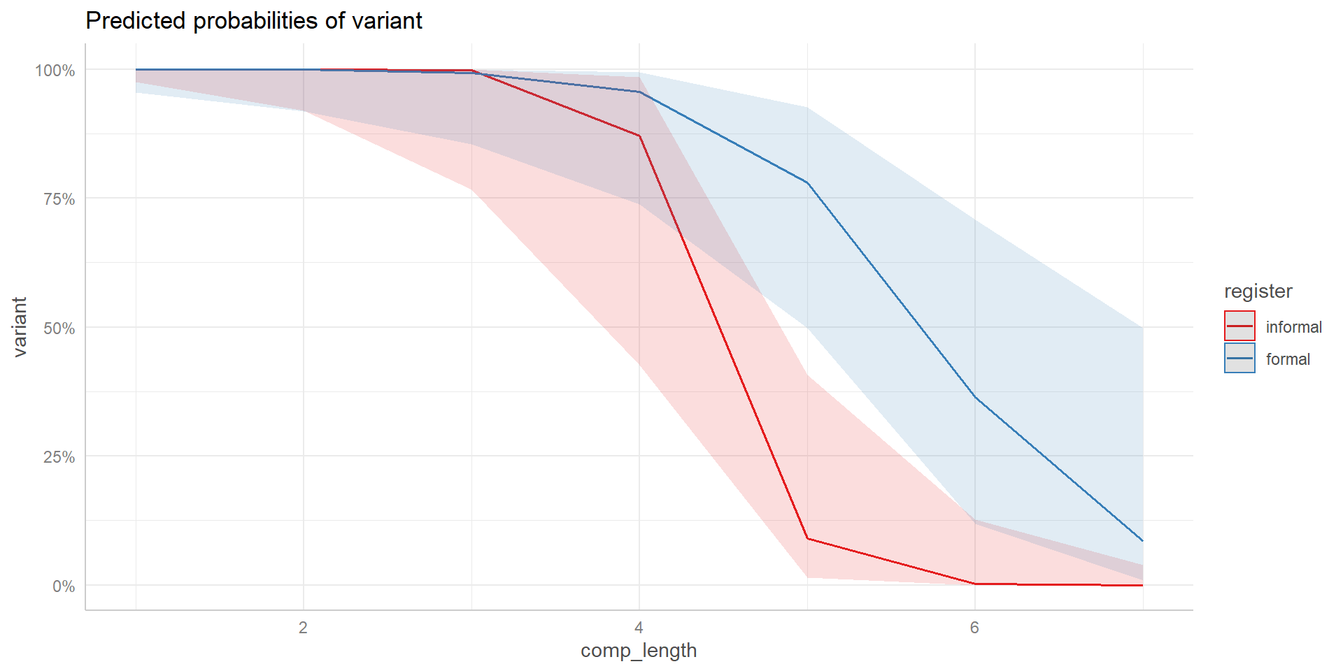
Possible interactions of complement length and register (is the text formal or informal?) on choice of gonna.

The effect of complement length is also positive/negative but stronger/weaker when texts are informal.
The effect of complement length is positive/negative when texts are informal, reversed when texts are formal.

Model with interactions

m3 <- glm(variant ~ comp_length*register, data = gt, family = binomial(logit))
summary(m3)


Call:
glm(formula = variant ~ comp_length * register, family = binomial(logit), 
    data = gt)

Deviance Residuals: 
    Min       1Q   Median       3Q      Max  
-2.5689  -0.0792  -0.0030   0.1584   1.8033  

Coefficients:
                           Estimate Std. Error z value Pr(>|z|)   
(Intercept)                   18.78       7.10    2.64   0.0082 **
comp_length                   -4.22       1.55   -2.72   0.0065 **
registerformal                -8.39       7.89   -1.06   0.2878   
comp_length:registerformal     2.39       1.67    1.43   0.1529   
---
Signif. codes:  0 '***' 0.001 '**' 0.01 '*' 0.05 '.' 0.1 ' ' 1

(Dispersion parameter for binomial family taken to be 1)

    Null deviance: 138.629  on 99  degrees of freedom
Residual deviance:  31.103  on 96  degrees of freedom
AIC: 39.1

Number of Fisher Scoring iterations: 8

Interpretation

Intercept is interpreted in the same way.
comp_length is the effect of complement length in informal register.
registerformal is the effect of the formal register at 0 complement length.
comp_length:registerformal is the difference in the effect of complement length in formal register, compared to informal register.

Visualization

Code

library(ggeffects)
plot(ggpredict(m3, c("comp_length", "register")))

Random effects

Fixed vs random effects

Unlike fixed effects (what we have dealt with up to now), random effects:

May not be replicable in a different dataset.
Involve a sample of the possible values in the population.

Examples: speaker, lexical effects, topic… → often operationalized as filename.

Random intercept

The intercept can vary.

Different individuals prefer gonna over going to regardless of complement length.
Certain children always produce longer utterances than others of the same age.

Nested random intercept

E.g. random intercept for filename and random intercept for register; each filename occurs in only one register.

Random slope

The slope of a fixed effect can vary.

A given predictor can have different effects in different texts.

Complement length is more influential in the choice of gonna for some individuals than for others.
For certain children, utterance length increases with age at a higher pace than of others.

How to

lme4::glmer() instead of glm(); lme4::lmer() instead of lm().
- The control argument helps us deal with convergence issues.

Extension of the R formula:
- (1 | filename) for filename as random effect.
- (age | child) for child as a random slope for age.

Model with random effects

m4 <- lme4::glmer(variant ~ comp_length*register + (1 | source), data = gt, family = binomial)
summary(m4)

Generalized linear mixed model fit by maximum likelihood (Laplace
  Approximation) [glmerMod]
 Family: binomial  ( logit )
Formula: variant ~ comp_length * register + (1 | source)
   Data: gt

     AIC      BIC   logLik deviance df.resid 
    40.7     53.7    -15.3     30.7       95 

Scaled residuals: 
   Min     1Q Median     3Q    Max 
-4.041 -0.031 -0.001  0.063  1.343 

Random effects:
 Groups Name        Variance Std.Dev.
 source (Intercept) 1.6      1.26    
Number of obs: 100, groups:  source, 26

Fixed effects:
                           Estimate Std. Error z value Pr(>|z|)  
(Intercept)                   23.19      11.72    1.98    0.048 *
comp_length                   -5.18       2.56   -2.03    0.043 *
registerformal               -10.30       9.77   -1.05    0.292  
comp_length:registerformal     2.94       2.18    1.35    0.177  
---
Signif. codes:  0 '***' 0.001 '**' 0.01 '*' 0.05 '.' 0.1 ' ' 1

Correlation of Fixed Effects:
            (Intr) cmp_ln rgstrf
comp_length -0.997              
registrfrml -0.829  0.827       
cmp_lngth:r  0.890 -0.894 -0.985

Compare models

Code

performance::compare_performance(m1, m2, m3, m4, metrics = "AIC")

# Comparison of Model Performance Indices

Name |    Model | AIC (weights)
-------------------------------
m1   |      glm |  51.6 (<.001)
m2   |      glm |  40.0 (0.303)
m3   |      glm |  39.1 (0.479)
m4   | glmerMod |  40.7 (0.217)

Next: Correspondence Analysis