Linear regression analysis
Methods of Corpus Linguistics (class 5)
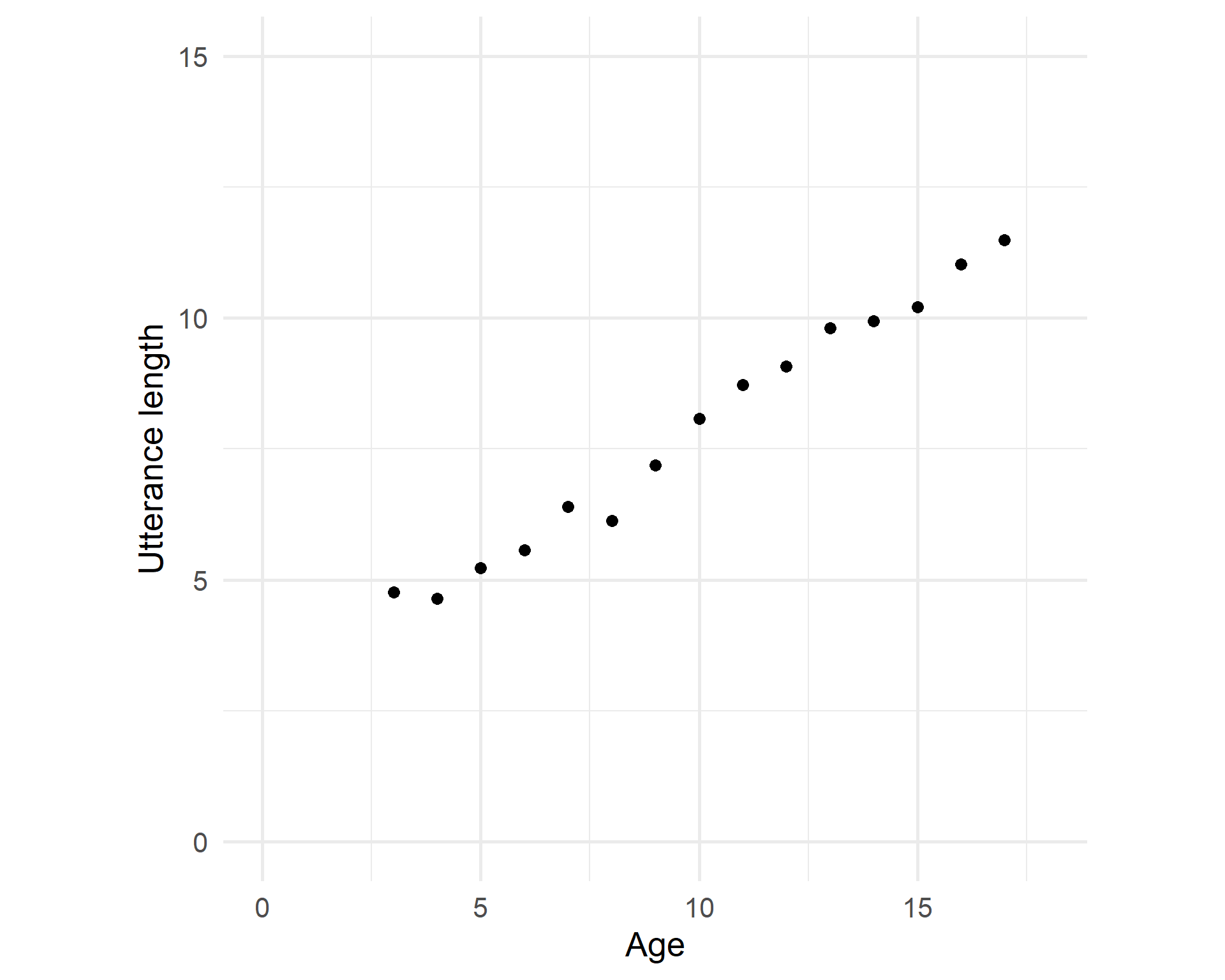
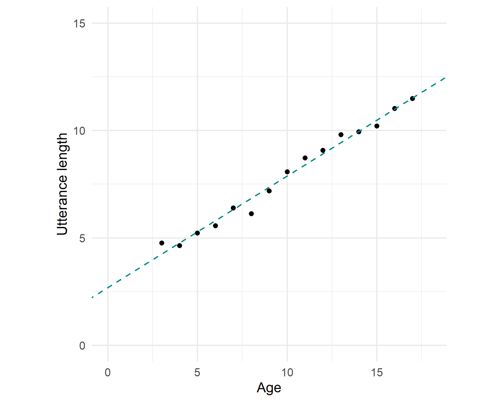
Scatterplot
What is the relationship between the age of a child and the mean length of their utterances (in a corpus)?
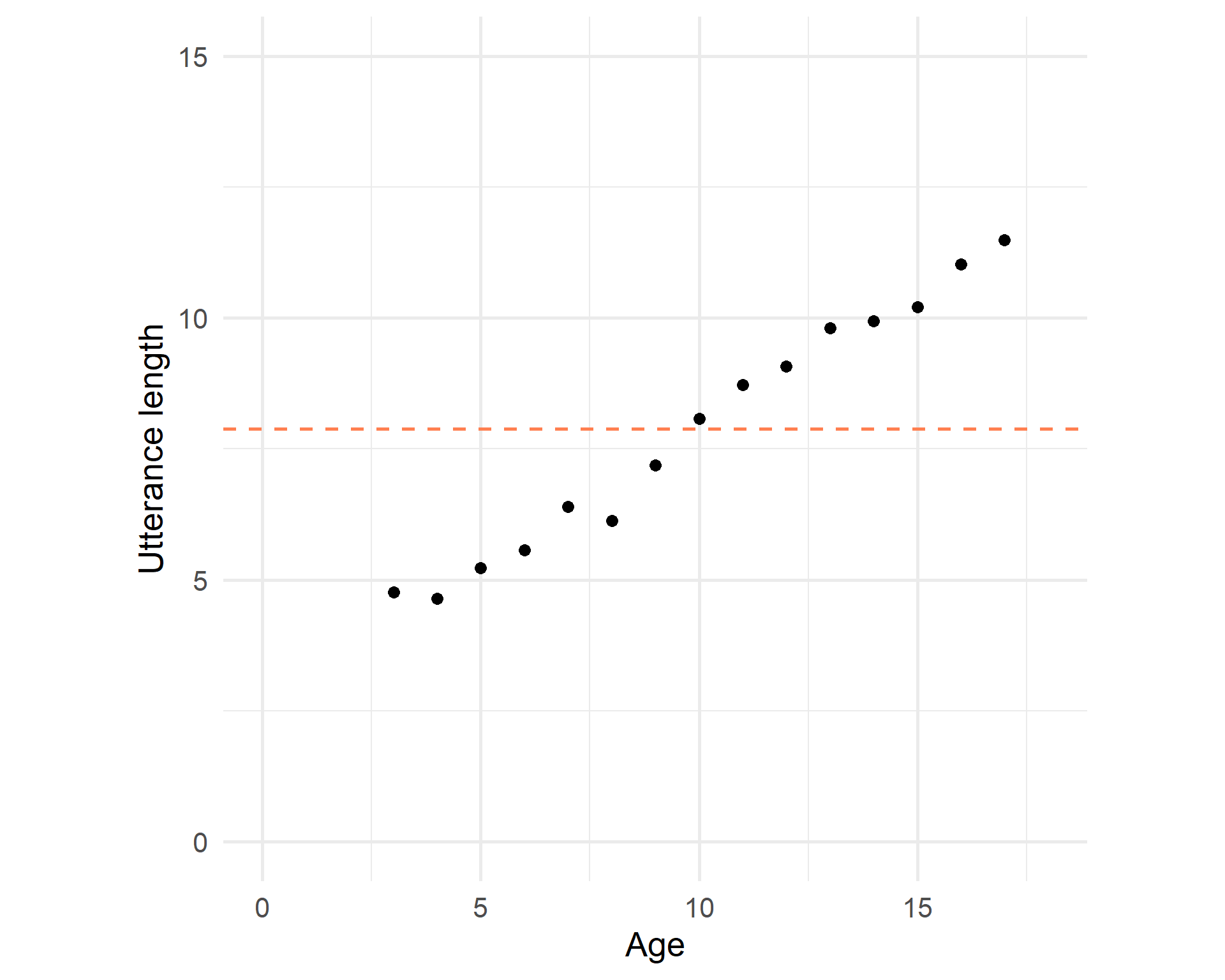
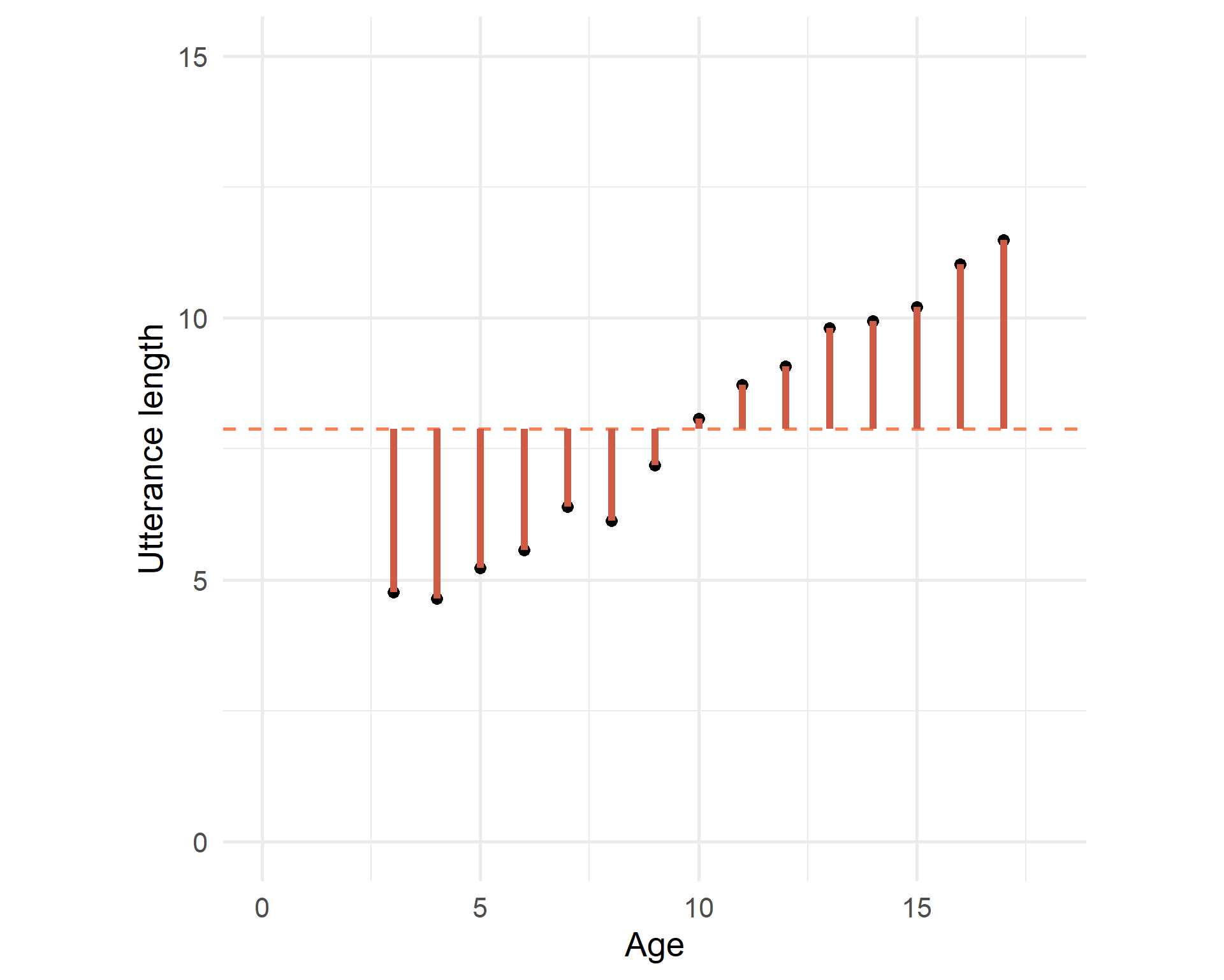
Intercept
The average utterance length is 7.885:
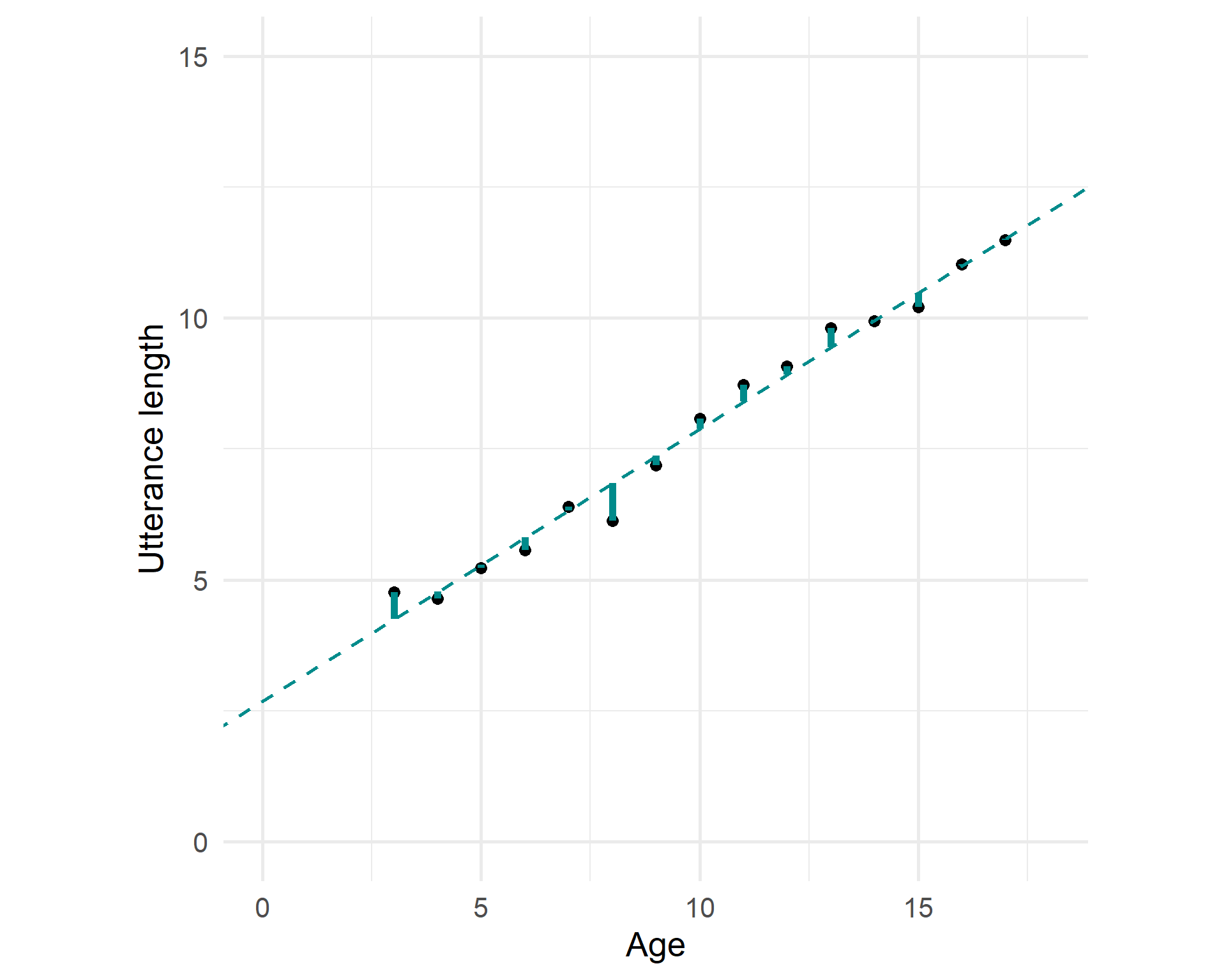
Fitted model
But we try to find a line that fits the trend the best:
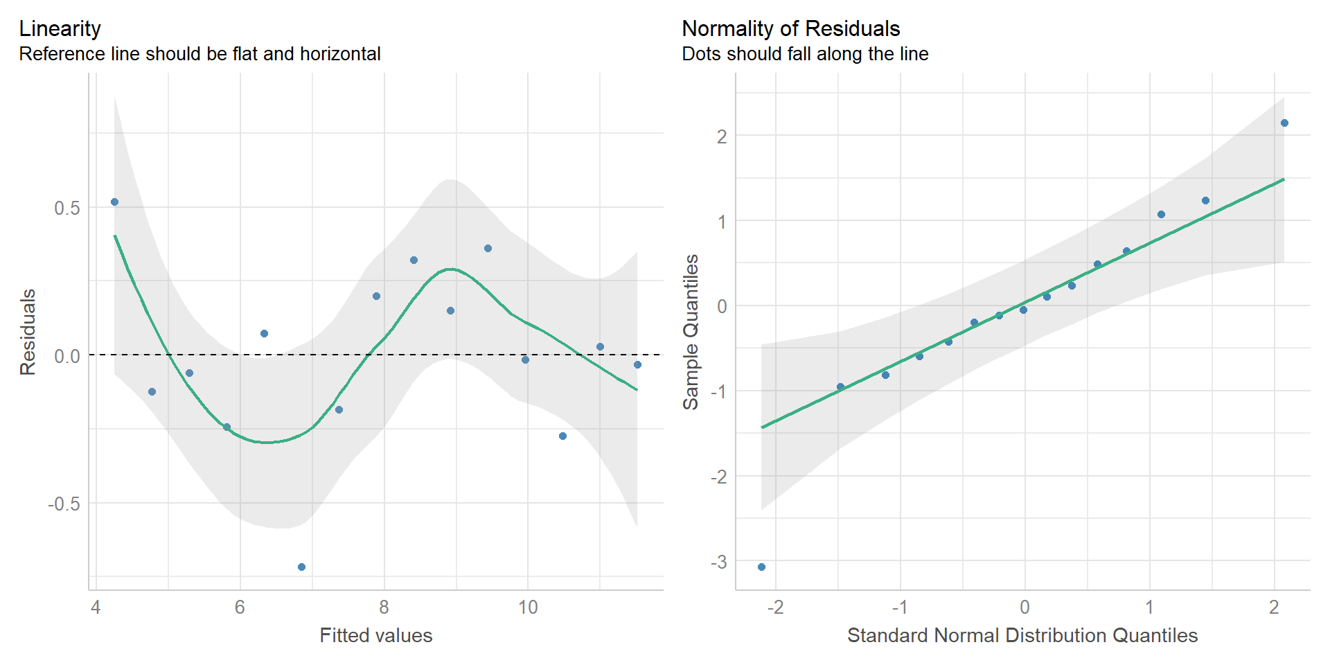
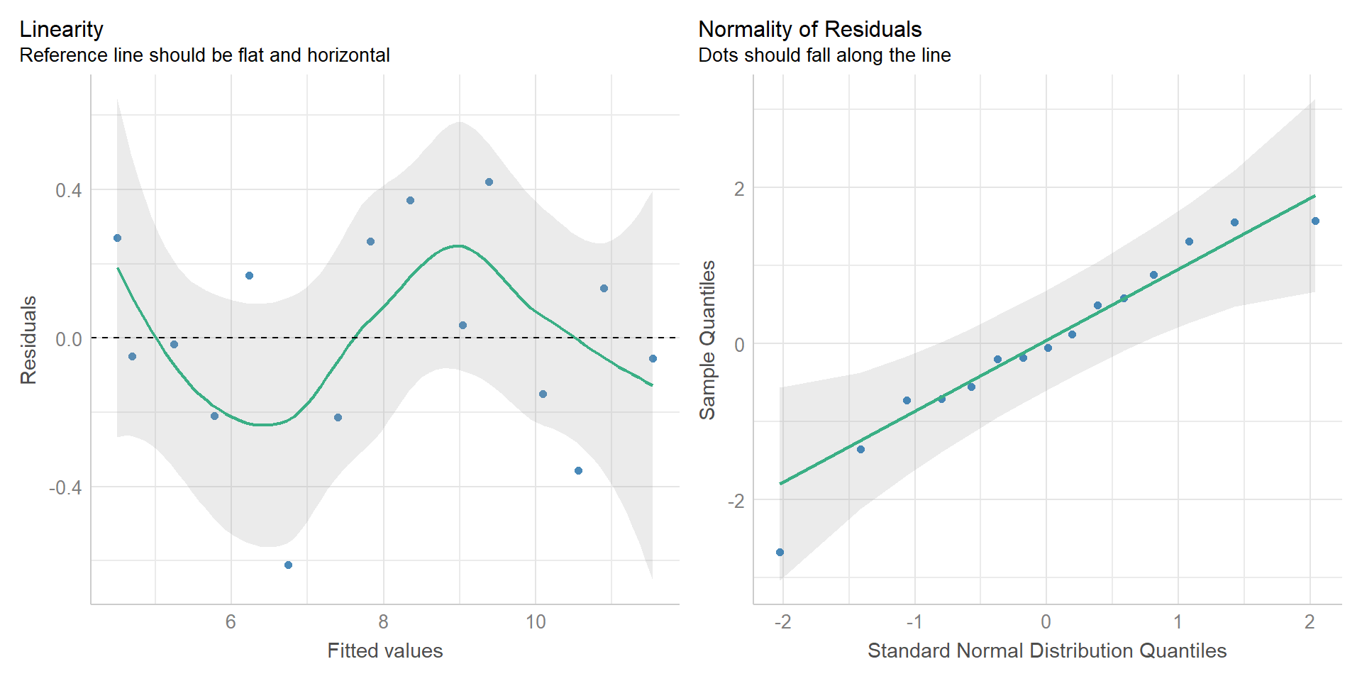
Error
Two levels: example
Code
ggplot(utt_lengths_cat, aes(x = as.numeric(mono)-1, y = utterance_length)) +
  geom_point(size = 3) + geom_smooth(method = "lm", se = FALSE, color = "darkolivegreen4") +
  labs(x = "Is the family monolingual?", y = "Utterance length") +
  ylim(c(0,15)) + scale_x_continuous(breaks = c(0, 1), labels = c("no", "yes")) +
  theme_minimal(base_size = 20) + theme(aspect.ratio = 1)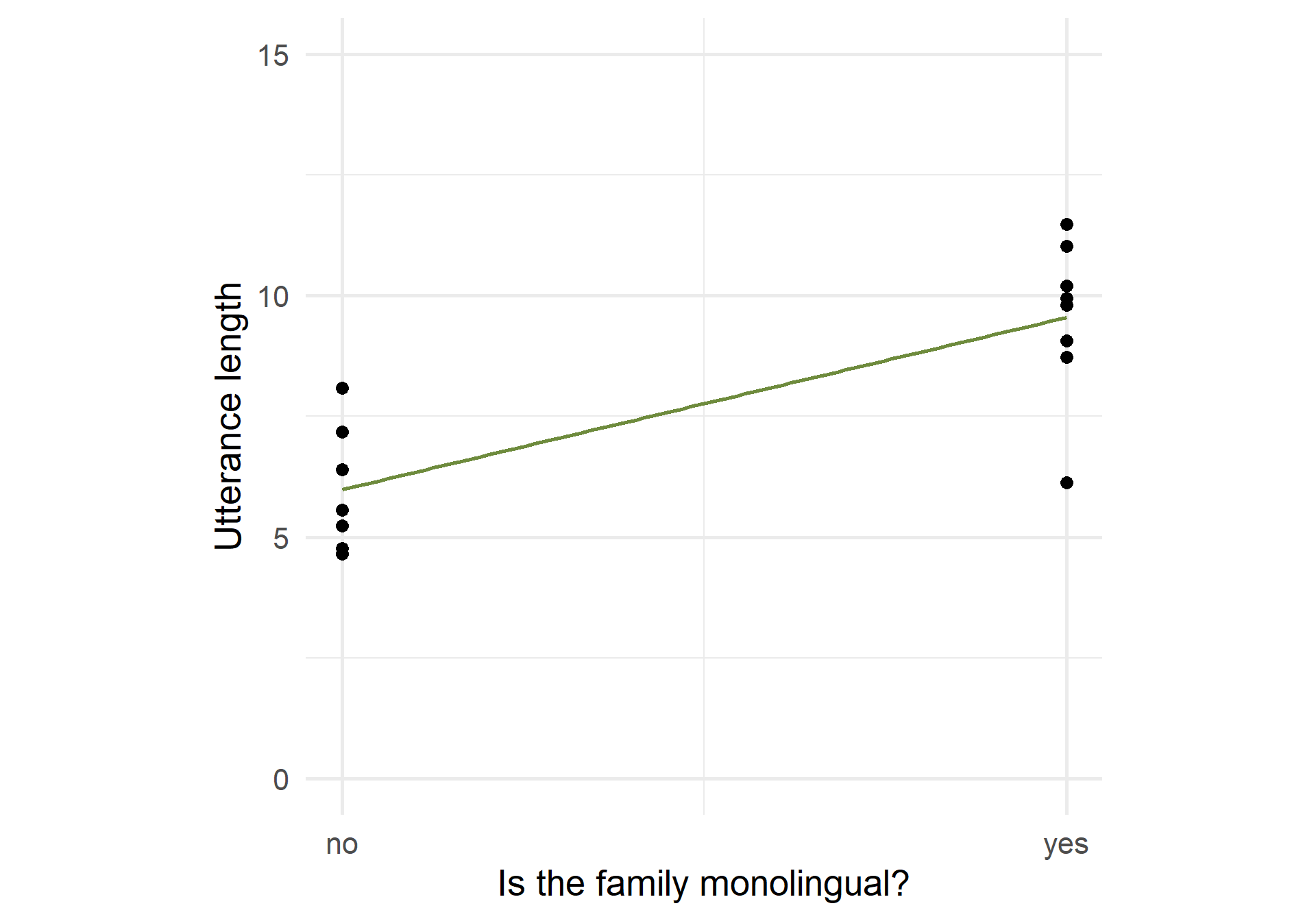
Call:
lm(formula = utterance_length ~ mono, data = utt_lengths_cat)

Residuals:
   Min     1Q Median     3Q    Max
-3.419 -0.788  0.253  0.928  2.100

Coefficients:
            Estimate Std. Error t value Pr(>|t|)
(Intercept)    5.983      0.566    10.6  9.5e-08 ***
monoyes        3.566      0.776     4.6    5e-04 ***
---
Signif. codes:  0 '***' 0.001 '**' 0.01 '*' 0.05 '.' 0.1 ' ' 1

Residual standard error: 1.5 on 13 degrees of freedom
Multiple R-squared:  0.619, Adjusted R-squared:  0.59
F-statistic: 21.1 on 1 and 13 DF,  p-value: 5e-04