Reading and exploring a corpus

Methods of Corpus Linguistics (class 2)

Mariana Montes

Outline

• Initialize project
• Add corpus
• Explore corpus
• Describe corpus

Initialize project

Steps

1. Create an R project, check on the “git repository” checkbox and commit changes

• Alternatively, run usethis::use_git()

2. Add remote on the terminal following the instructions on GitHub (see next slide).

In the future

For future projects, the workflow may be different; check Happy Git With R for a guide.

Connect repository to GitHub

This only needs to be done once at the beginning.

git remote add origin <url>
git branch -M main
git push -u origin main

Note

<url> is the url of your repository.

Notes

• If you make changes on the remote, use git pull before making changes in the local repo.

• Avoid .RData with Tools > Global Options > General > Workspace/History

• You can work with Git(Hub) on the Git tab of RStudio or on the Git Bash Terminal

Add corpus

Git branch

Optionally, you can start “new work” on a new branch and then merge it to main.

git branch explore-corpus
git checkout explore-corpus

Tip

I will only look at what you push to the main branch.

Add a folder with a corpus

Download the corpora from Toledo (mcl.zip file with various corpora) and copy/move the brown folder to your project. There are different options.

• Top level
• Corpus/corpora folder
• Data folder

To be accessed with here::here("brown").

project
|_brown
|_project.Rproj
|_.gitignore

To be accessed with here::here("corpus", "brown").

project
|_corpus
| \_brown
|_project.Rproj
|_.gitignore

To be accessed with here::here("data", "corpus", "brown").

project
|_data
| \_corpus
|   \_brown
|_project.Rproj
|_.gitignore

.gitignore

We don’t want to track the corpus on git (because of size and licenses).

1. Open .gitignore.

2. Add a line for the folder to ignore, e.g. /brown/.

(Check git status!)

Explore corpus

Create new R script

• Easier to run the code again and to share it.

• Load packages first.

• Do not change your working directory; use here() or reliable relative paths.

Tip

You can add comments to explain what you did and even hierarchical sections!

Start of the script

# Load packages ----
library(here)
library(tidyverse)
library(mclm)

# Load data ----
path_to_corpus <- here("studies", "_corpora", "brown") # adapt

## List filenames ----
brown_fnames <- get_fnames(path_to_corpus)

Inspect objects

In the console:

• path_to_corpus = print(path_to_corpus)
• print(brown_fnames, hide_path = path_to_corpus)
• explore(brown_fnames)
• drop_re(brown_fnames, "/c[a-z]")

Create a frequency list

Create it on the script, inspect in the console (or from the script).

brown_fnames <- brown_fnames %>% 
  keep_re("/c[a-z]")
flist <- freqlist(brown_fnames, re_token_splitter = re("\\s+"))

Tip

Check out the “freqlists” tutorial of {mclmtutorials} (learnr::run_tutorial("freqlists", "mclmtutorials")) to learn why we need the re_token_splitter argument.

Explore the frequency list

print(flist, n = 3)

Frequency list (types in list: 63517, tokens in list: 1162192)
rank   type abs_freq nrm_freq
---- ------ -------- --------
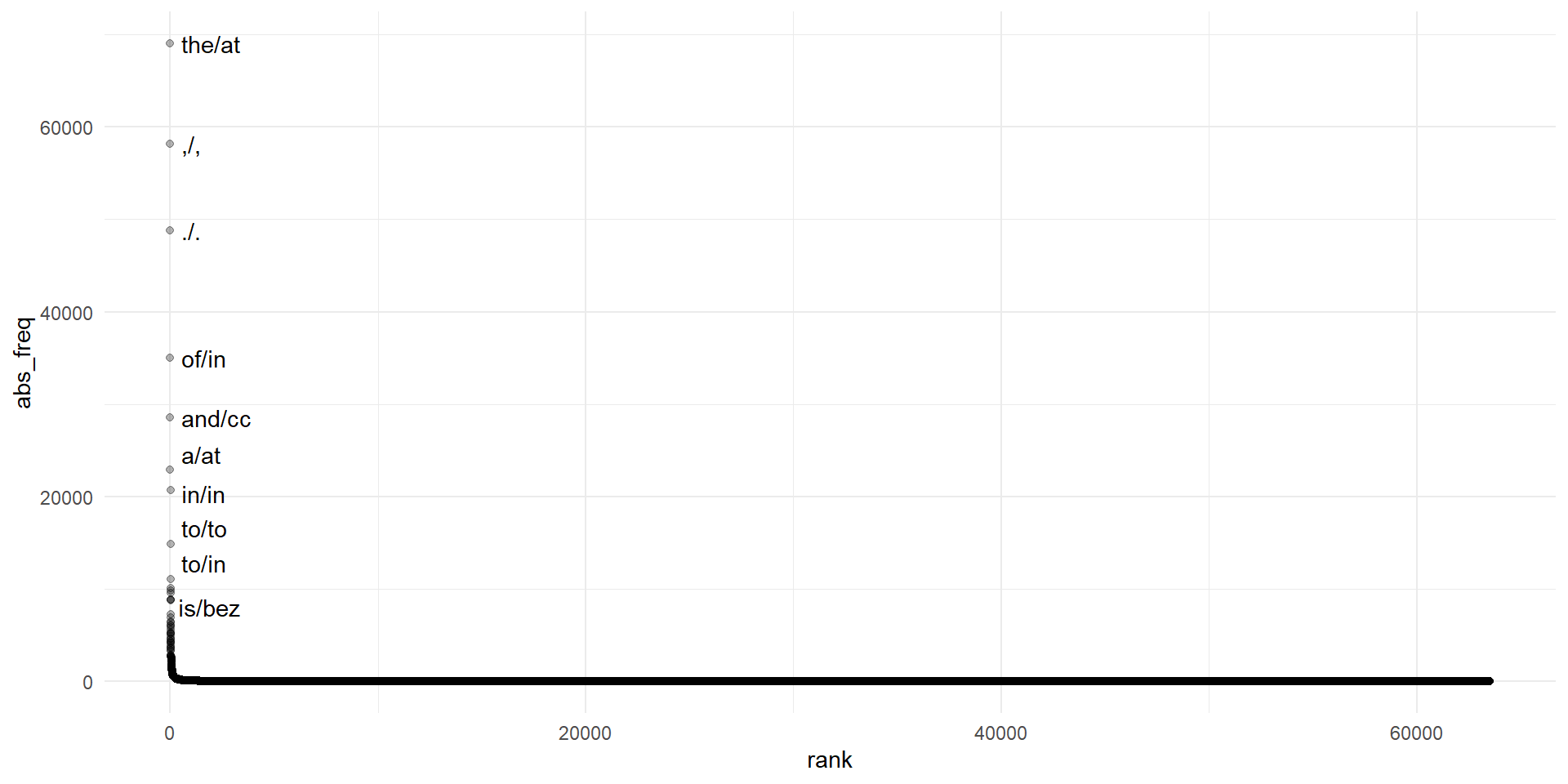
   1 the/at    69013  593.818
   2    ,/,    58153  500.373
   3    ./.    48812  419.999
...

n_tokens(flist)

[1] 1162192

n_types(flist)

[1] 63517

Tip

Check out the documentation

Plot frequencies I

as_tibble(flist) %>% 
  ggplot(aes(x = rank, y = abs_freq)) +
  geom_point(alpha = 0.3) +
  theme_minimal()

Plot frequencies II

as_tibble(flist) %>% 
  ggplot(aes(x = rank, y = abs_freq)) +
  geom_point(alpha = 0.3) +
  ggrepel::geom_text_repel(data = as_tibble(keep_bool(flist, flist > 10000)),
                  aes(label = type), xlim = c(0, NA)) +
  theme_minimal()

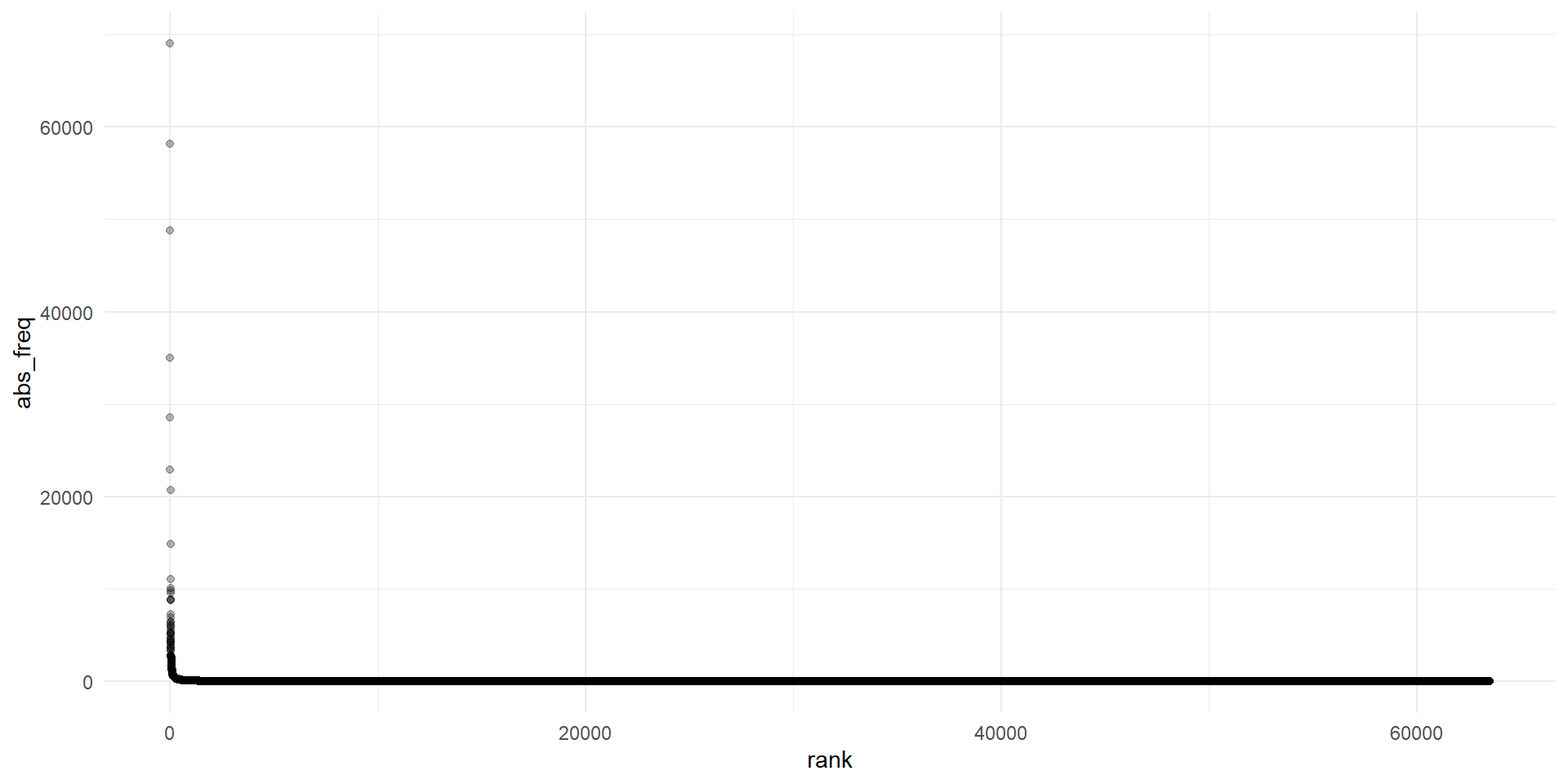
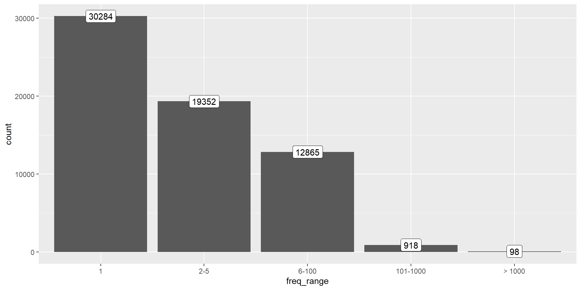
Plot frequencies III

as_tibble(flist) %>%
  mutate(freq_range = case_when(
    abs_freq == 1 ~ "1",
    abs_freq <= 5 ~ "2-5",
    abs_freq <= 100 ~ "6-100",
    abs_freq <= 1000 ~ "101-1000",
    TRUE ~ "> 1000"
  ) %>% fct_reorder(abs_freq)) %>% 
  ggplot(aes(x = freq_range)) +
  geom_bar() +
  geom_label(stat = "count", aes(label = ..count..))

Plot frequencies III

Describe corpus

Read the documentation

It might be in a README file, online, as a paper…

• What time period(s) is/are covered?

• What genre(s)? Language varieties?

• Written? Transcripts of oral texts?

• Is it a monitor corpus?

Licenses

Check also the permissions you have as user of the corpus.

Quarto document

• Create basic Quarto document

• Set meta data on the YAML choosing output

• Optional: render to check it’s working

• Remove current text and write your own

Code in a Quarto document

• Inline code surrounded by backticks and starting with “r”.

• Code chunks: to run arbitrary code, create tables and plots, print glosses with {glossr}.

• Read external scripts with source() or with the code or file chunk options.

Inline code

Markdown

The Brown corpus used in this project has `r prettyNum(n_tokens(flist))` tokens
and `r n_types(flist)` types,
giving us a type-token ratio of `r round(n_types(flist)/n_tokens(flist), 2)`.

Output

The Brown corpus used in this project has 1162192 tokens and 63517 types, giving us a type-token ratio of 0.05.

Code chunks

tbl <- (flist) %>% head(5)
tbl

Frequency list (types in list: 5, tokens in list: 239548)
<total number of tokens: 1162192>
rank orig_rank   type abs_freq nrm_freq
---- --------- ------ -------- --------
   1         1 the/at    69013  593.818
   2         2    ,/,    58153  500.373
   3         3    ./.    48812  419.999
   4         4  of/in    35028  301.396
   5         5 and/cc    28542  245.588

Tables with knitr::kable()

library(knitr)
tbl <- (flist) %>% head(5)
tbl %>% 
  kable()

Table 1: Top 5 types and their frequencies.

rank	orig_rank	type	abs_freq	nrm_freq
1	1	the/at	69013	593.8175
2	2	,/,	58153	500.3734
3	3	./.	48812	419.9994
4	4	of/in	35028	301.3960
5	5	and/cc	28542	245.5876

Tables with kableExtra::kbl()

library(kableExtra)
tbl <- (flist) %>% head(5)
tbl %>% 
  kbl() %>% 
  kable_paper()

Table 2: Top 5 types and their frequencies.

rank	orig_rank	type	abs_freq	nrm_freq
1	1	the/at	69013	593.8175
2	2	,/,	58153	500.3734
3	3	./.	48812	419.9994
4	4	of/in	35028	301.3960
5	5	and/cc	28542	245.5876

Import code

In both cases, you might want to use the include: false chunk option to avoid printing neither the code itself or its output.

• The code
• source()
• file
• code=readLines

# script.R    
x <- "New variable called x"    
print(x)    

```{r}
#| label: setup-chunk
source(here::here("R", "script.R"), local = knitr::knit_global())
```

[1] "New variable called x"

```{r}
#| label: file
#| file: !expr here::here("R", "script.R")
x <- "New variable called x"
print(x)
```

[1] "New variable called x"

```{r}
#| label: code
#| code: !expr readLines(here::here("R", "script.R"))
x <- "New variable called x"
print(x)
```

[1] "New variable called x"

Stage, commit, push

• Commit whenever you reach a “stage”.
• Push at most once a day.

git status
git add .
git commit -m "my first quarto document"
git push

Branches and remotes

The first time you try to push from a local branch you may get an error! Just follow the instructions, don’t panic :)

From a branch

If you were in your explore-corpus branch and want to bring changes to main

• git merge
• git checkout

main is now totally up-to-speed.

git checkout main
git merge explore-corpus

Get only selected folders/files.

git checkout main
git checkout explore-corpus script.R

Next: Contingency tables